- 功能描述:获取A股每日的筹码分布情况,提供各价位占比
- 返回限量:单次请求最大返回6000行
- 接口权限:5000积分每天限量20000次每分钟限量200次,10000积分每天限量200000次每分钟限量500次,15000积分每天不限总量每分钟限量1000次
- 说明:
1. 每日18~21点更新;
2. 数据最早从2018年开始;
输入参数:
名称 |
类型 |
必选 |
描述 |
ts_code |
str |
Y |
股票代码 |
trade_date |
str |
N |
交易日期(YYYYMMDD) |
start_date |
str |
N |
开始日期 |
end_date |
str |
N |
结束日期 |
输出参数:
名称 |
类型 |
默认显示 |
描述 |
ts_code |
str |
Y |
股票代码 |
trade_date |
str |
Y |
交易日期 |
price |
float |
Y |
成本价格 |
percent |
float |
Y |
价格占比(%) |
示例:
示例1:获取某支股票某个交易日的筹码分布
通过传递ts_code可用于指定特定的股票,传递trade_date可用于指定交易日期。
import tushare as ts
pro = ts.pro_api()
df = pro.cyq_chips(ts_code='600000.SH', trade_date='20260723')
df
输出结果:
          ts_code        trade_date        price        percent
0        600000.SH        20260723        0.5        0.01
1        600000.SH        20260723        0.6        0.01
2        600000.SH        20260723        0.7        0.01
3        600000.SH        20260723        0.8        0.01
4        600000.SH        20260723        0.9        0.01
...        ...        ...        ...        ...
129        600000.SH        20260723        13.4        1.03
130        600000.SH        20260723        13.5        3.43
131        600000.SH        20260723        13.6        2.10
132        600000.SH        20260723        13.7        0.56
133        600000.SH        20260723        13.8        0.72
134 rows × 4 columns
示例2:绘制筹码分布图
一张标准的筹码分布图通常包含以下几个关键指标:
a、筹码柱(筹码峰)
筹码分布图由无数根水平柱状条构成,每一根柱子代表一个具体价位上的筹码数量(占比)。柱子越长,说明该价位成交越密集、持仓的人越多。多个相邻的密集柱子会形成筹码峰——这是市场平均成本最集中的区域,也是重要的支撑位或压力位。
b、获利比例
获利比例是指当前股价以下(即买入成本低于当前市价)的筹码占总筹码的百分比。数值越大,说明市场上获利的人越多,但也意味着潜在的抛压可能越大。
c、平均成本
平均成本是所有持仓筹码的加权平均价格,反映了市场整体的持仓成本水平。当股价高于平均成本时,市场整体处于盈利状态;反之则整体亏损。
d、支撑位与压力位
这是筹码分布中最重要的两个定位指标:
- 支撑位 = 总获利盘的筹码平均价:当股价跌到这个位置时,大部分持仓者仍处于盈利状态,会激发“抄底”心理和“惜售”情绪,从而对股价形成支撑。
- 压力位 = 总套牢盘的筹码平均价:当股价涨到这个位置时,意味着大部分之前被套牢的投资者刚刚解套,会引发强烈的“解套卖出”意愿,形成巨大的抛售压力。
e、筹码集中度
筹码集中度衡量筹码分布在一个价格区间内的密集程度,数值越小说明筹码越集中。
常见的计算公式为:
筹码集中度=(区间上轨−区间下轨)/(区间上轨+区间下轨)
筹码集中度 = (区间上轨 - 区间下轨) / (区间上轨 + 区间下轨)
其中,90%筹码集中度是去掉价格最高5%和最低5%的“极端”筹码后,中间90%筹码所在区间的集中度。集中度小于10%通常被视为筹码高度密集的信号。
f、90%筹码区间与70%筹码区间
- 90%筹码区间:去掉最高5%和最低5%的筹码后,中间90%筹码分布的价格范围
- 70%筹码区间:去掉最高15%和最低15%的筹码后,中间70%筹码分布的价格范围
- 区间重合度:是指90%筹码区间和70%筹码区间的重合比例。两个区间的筹码重合度越高,说明筹码成本越集中,股价波动幅度越小。
这两个区间越窄,说明筹码越集中;区间越宽,说明市场成本越分散。
下面给出绘图代码:
import tushare as ts
import pandas as pd
import numpy as np
import matplotlib.pyplot as plt
from matplotlib import gridspec
# 设置中文字体
plt.rcParams['font.sans-serif'] = ['SimHei', 'Microsoft YaHei', 'Arial Unicode MS']
plt.rcParams['axes.unicode_minus'] = False
def get_chips_data(pro, ts_code, trade_date):
    """获取筹码分布数据和当日收盘价"""
    df_chips = pro.cyq_chips(ts_code=ts_code, trade_date=trade_date)
    if df_chips.empty:
        raise ValueError(f"未获取到 {ts_code} 在 {trade_date} 的筹码数据")
    df_daily = pro.daily(ts_code=ts_code, trade_date=trade_date)
    if df_daily.empty:
        raise ValueError(f"未获取到 {ts_code} 在 {trade_date} 的日线行情")
    close = df_daily.iloc[0]['close']
    return df_chips, close
def calc_cost_percentile(df_sorted, p):
    """计算累计筹码占比达到 p% 对应的价格(线性插值)"""
    cumsum = np.cumsum(df_sorted['percent'].values)
    if p <= 0:
        return df_sorted.iloc[0]['price']
    if p >= 100:
        return df_sorted.iloc[-1]['price']
    idx = np.searchsorted(cumsum, p)
    if idx == 0:
        return df_sorted.iloc[0]['price']
    if idx >= len(df_sorted):
        return df_sorted.iloc[-1]['price']
    price_low = df_sorted.iloc[idx-1]['price']
    price_high = df_sorted.iloc[idx]['price']
    cum_low = cumsum[idx-1]
    cum_high = cumsum[idx]
    if cum_high == cum_low:
        return price_low
    return price_low + (price_high - price_low) * (p - cum_low) / (cum_high - cum_low)
def plot_chips(ts_code, trade_date,
               p_low=5, p_high=95,
               p_low_70=15, p_high_70=85,
               display_p_low=0, display_p_high=100,
               min_percent_filter=0.0):
    """
    绘制筹码分布图(水平柱状图)
    参数:
        ts_code: 股票代码,如 '000001.SZ'
        trade_date: 交易日期,格式 'YYYYMMDD'
        token: Tushare token(可选)
        p_low: 90%区间下轨百分位(默认5)
        p_high: 90%区间上轨百分位(默认95)
        p_low_70: 70%区间下轨百分位(默认15)
        p_high_70: 70%区间上轨百分位(默认85)
        display_p_low: 显示下限百分位(默认0)
        display_p_high: 显示上限百分位(默认100)
        min_percent_filter: 过滤筹码占比低于此值的价格点(默认0.0)
    """
    pro = ts.pro_api()
    # 获取全量数据
    df_full, close = get_chips_data(pro, ts_code, trade_date)
    if min_percent_filter > 0:
        df_full = df_full[df_full['percent'] >= min_percent_filter]
    df_full = df_full.sort_values('price').reset_index(drop=True)
    prices_full = df_full['price'].values
    percents_full = df_full['percent'].values
    # ---- 1. 计算各项指标(基于全量数据) ----
    # 平均成本
    avg_cost = np.sum(prices_full * percents_full) / 100.0
    # 获利比例
    profit_ratio = np.sum(percents_full[prices_full <= close])
    # 90% 和 70% 筹码区间
    low_90 = calc_cost_percentile(df_full, p_low)
    high_90 = calc_cost_percentile(df_full, p_high)
    low_70 = calc_cost_percentile(df_full, p_low_70)
    high_70 = calc_cost_percentile(df_full, p_high_70)
    range_90 = high_90 - low_90
    range_70 = high_70 - low_70
    overlap_ratio = range_70 / range_90 if range_90 > 0 else np.nan
    concentration_90 = (high_90 - low_90) / (high_90 + low_90) if (high_90 + low_90) > 0 else np.nan
    # 支撑位 = 获利盘的平均成本(价格 < 收盘价的筹码加权均价)
    profit_mask = prices_full < close
    if np.any(profit_mask):
        profit_prices = prices_full[profit_mask]
        profit_percents = percents_full[profit_mask]
        if np.sum(profit_percents) > 0:
            support = np.sum(profit_prices * profit_percents) / np.sum(profit_percents)
        else:
            support = prices_full[0]  # 无有效获利筹码时,取最低价
    else:
        support = prices_full[0]  # 全部套牢,最低价为支撑
    # 压力位 = 套牢盘的平均成本(价格 > 收盘价的筹码加权均价)
    loss_mask = prices_full > close
    if np.any(loss_mask):
        loss_prices = prices_full[loss_mask]
        loss_percents = percents_full[loss_mask]
        if np.sum(loss_percents) > 0:
            resistance = np.sum(loss_prices * loss_percents) / np.sum(loss_percents)
        else:
            resistance = prices_full[-1]  # 无有效套牢筹码时,取最高价
    else:
        resistance = prices_full[-1]  # 全部获利,最高价为压力
    # ---- 2. 准备绘图数据(仅用于显示) ----
    price_min_display = calc_cost_percentile(df_full, display_p_low)
    price_max_display = calc_cost_percentile(df_full, display_p_high)
    mask = (df_full['price'] >= price_min_display) & (df_full['price'] <= price_max_display)
    if min_percent_filter > 0:
        mask = mask & (df_full['percent'] >= min_percent_filter)
    df_display = df_full[mask].copy()
    if df_display.empty:
        print("警告:应用显示过滤后无数据可绘,将显示全部数据")
        df_display = df_full.copy()
    prices_display = df_display['price'].values
    percents_display = df_display['percent'].values
    # ---- 3. 绘制 ----
    fig = plt.figure(figsize=(14, 8))
    gs = gridspec.GridSpec(1, 2, width_ratios=[0.7, 0.3])
    ax = plt.subplot(gs[0])
    # 柱子高度
    if len(prices_display) > 1:
        gaps = np.diff(prices_display)
        min_gap = np.min(gaps)
        if min_gap == 0:
            min_gap = (prices_display[-1] - prices_display[0]) / max(1, len(prices_display)-1)
        bar_height = min_gap
    else:
        bar_height = 0.01
    # 颜色
    colors = []
    for p in prices_display:
        if p > close:
            colors.append('green')
        elif p < close:
            colors.append('red')
        else:
            colors.append('gray')
    ax.barh(
        y=prices_display,
        width=percents_display,
        height=bar_height,
        color=colors,
        edgecolor='none',
        alpha=0.8
    )
    # ---- 4. 标注线(使用新的支撑位和压力位) ----
    ax.axhline(y=avg_cost, color='blue', linestyle='--', linewidth=1.5, label=f'平均成本 {avg_cost:.2f}')
    ax.axhline(y=support, color='orange', linestyle='-.', linewidth=1.5, label=f'支撑位 {support:.2f} (获利盘均价)')
    ax.axhline(y=resistance, color='purple', linestyle='-.', linewidth=1.5, label=f'压力位 {resistance:.2f} (套牢盘均价)')
    ax.axhline(y=close, color='black', linestyle='-', linewidth=0.8, alpha=0.5, label=f'收盘价 {close:.2f}')
    ax.set_xlabel('筹码占比 (%)', fontsize=16)
    ax.set_ylabel('价格 (元)', fontsize=16)
    ax.set_title(f'{ts_code} 筹码分布图 ({trade_date})', fontsize=20)
    ax.grid(True, axis='x', alpha=0.3, linestyle=':')
    ax.tick_params(axis='both', labelsize=14)
    ax.legend(loc='upper right', fontsize=14)
    ax.yaxis.set_major_formatter(plt.FormatStrFormatter('%.2f'))
    # ---- 5. 右侧指标文本 ----
    ax_text = plt.subplot(gs[1])
    ax_text.axis('off')
    text_lines = [
        "【成本指标】",
        f"获利比例: {profit_ratio:.2f}%",
        f"压力位: {resistance:.2f}",
        f"平均成本: {avg_cost:.2f}",
        f"支撑位: {support:.2f}",
        "",
        "【集中度指标】",
        f"90%筹码区间: [{low_90:.2f}, {high_90:.2f}]",
        f"70%筹码区间: [{low_70:.2f}, {high_70:.2f}]",
        f"区间重合度: {overlap_ratio:.2%}" if not np.isnan(overlap_ratio) else "区间重合度: --",
        f"90%筹码集中度: {concentration_90:.2%}" if not np.isnan(concentration_90) else "90%筹码集中度: --"
    ]
    y_pos = 0.95
    for line in text_lines:
        ax_text.text(0.1, y_pos, line, fontsize=16, verticalalignment='top')
        y_pos -= 0.06
    plt.tight_layout()
    plt.show()
    # 返回所有指标
    return {
        'avg_cost': avg_cost,
        'profit_ratio': profit_ratio,
        'support': support,
        'resistance': resistance,
        'low_90': low_90,
        'high_90': high_90,
        'low_70': low_70,
        'high_70': high_70,
        'overlap_ratio': overlap_ratio,
        'concentration_90': concentration_90
    }
# ========== 使用示例 ==========
if __name__ == "__main__":
    plot_chips('000001.SZ', '20260723',
           display_p_low=2, display_p_high=98,
           min_percent_filter=0.01)
输出结果:
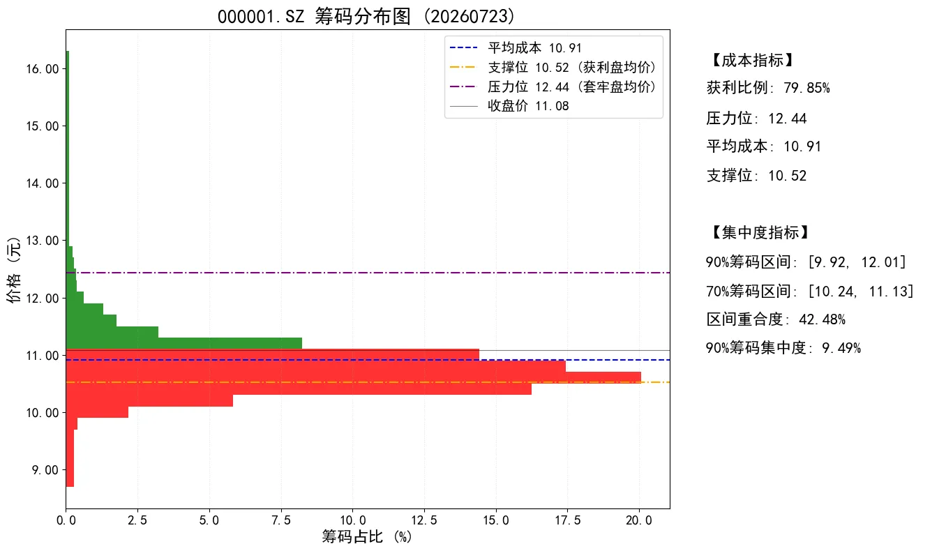
说明:
本文说明
本文旨在对Tushare的每日筹码分布cyq_chips数据接口进行介绍,提供更多参考示例和使用说明。
通过本接口可获取A股每日的筹码分布情况,提供各价位占比。本文介绍了如何获取某支股票某个交易日的筹码分布,介绍了标准筹码分布图中的关键指标,以及绘制了一张筹码分布图。
本文目的是为了让用户和AIGC工具能够更便捷、准确地使用该接口。大家在使用过程中遇到什么问题和建议可在线留言,作者会进行数据探索将结果更新到文章中,并将建议反馈给Tushare团队。本文另一个目的也是为了聚集大家的智慧以创建“我为人人,人人为我”的共创氛围。